|
This project is small demonstration of object detection and recognition using classical computer vision and machine learning. To put it simply, a computer vision technique called 'Histogram of Oriented Gradients' was used for creating feature vectors which were used to train a model. Then the test images were classified into 'phone' and 'not phone'. |
|
First and foremost the dataset needs to be classified into positive and negative images. The positive images are those that contain only the object that is to be detected. The negative images are a collection of images that contain anything but the object to be detected. Generally the number of negative images should be greater than the number of positive images. The dataset can be divided in a ratio of 60:20:20 for training, validation and testing (recommended) or just 80:20 for training and testing. |
|
|
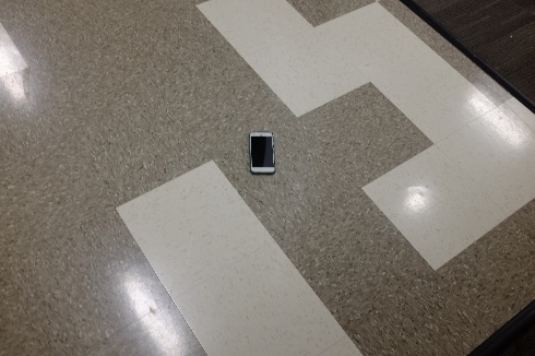
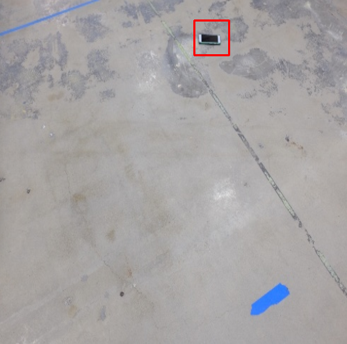
The image to be classified looks something like the picture above. The size of the object is quite small compared to the background. First the image is resized such that the height and width of the image are same. The positive image is cropped from this image and that part is replaced with a mask to get the negative image. Now, before finding the HOG feature vector, for each image, the negative image is divided into multiple grids such that size of each grid is the same as that of the positive image. |
|

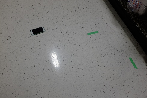
Positive image |
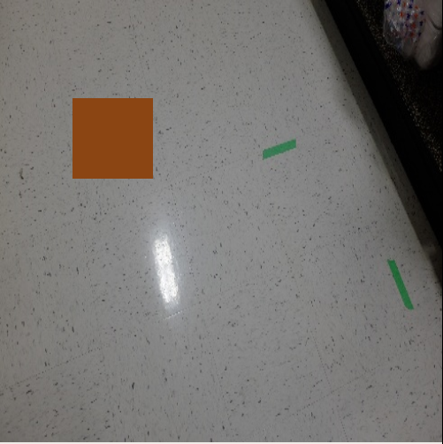
Negative image. The brown part is the mask |
|
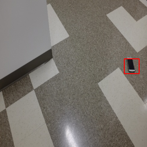
Once the preprocessing is done, the HOG Feature vectors are created for these images. Go to the link for a good resource to understand how the Histogram of Oriented Gradients work. After getting the HOG feature vectors for these images, they are fed to a Support Vector Classifier using the scikit-learn. A short intro to SVM. We have used polynomial kernel of degree 3. It performed the best out of all. This fits the data to a model that can be later used predict whether the object to be detected (phone) is present in the image or not. But the work is not yet done. The model still contains a lot false positives. In order to get rid of the same, we use a method called Hard Negative Mining. As the name suggests, we mine for false positives, i.e. those images that actually don't contain the object yet have been identified as positive by our model. So we run a predictor using the model we just created on the negative images. And the images for which we get the predictor output as positive image, we add that image's feature vector to the negative feature vectors and again train the model. Now the new trained model is robust to false positives. This model is saved as a .joblib file that can be imported later for predicting whether the phone is present or not. Now for detecting whether a phone is present in a given image or not, the image is again divided into same number of grids like the traning stage. HOG feature vectors are found for all the grids and fed to the model for prediction. If prediction is false for all the grids, then it means that the phone is not observed in the image. If there are multiple adjoining grid cells with prediction true, the cell with maximum probability is selected as the location of the phone. |
|
|
|
The accuracy without the hard negative mining was about 64% and that with the hard negative mining was almost 96%. |