|
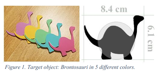
In this project I tried using classical geometry based computer vision for detecting 2-d colored brontosaurus. Figure 1 depicts the target object that has dimensions of 8.4X6.1. Due to its highly 2-dimensional shape, the thickness can be omitted from our models (4mm). |
|
|
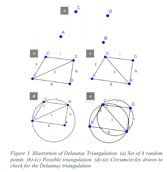
Triangulation is a method that is generally used for pathfinding algorithms. If there is a set of points in a plane and the path has to be found to traverse from one point to the other, triangulating these points helps find the required path. One of the triangulation methods, Delaunay triangulation, can be used for object detection. Delaunay Triangulation: The triangulation, f(t), of a set of discrete points P in a plane, is said to be Delaunay Triangulation iff no point in P is inside or on the circumcircle of any triangle of f(t), except the triangle vertices themselves. If this condition is fulfilled, then the triangulation is always unique for the set of points [1]. For instance, if there are 4 points as shown below, there are two possible ways of forming triangles as shown in Fig 3(b) and 3(c). However, if the circumcircles are drawn for both cases, it can be seen that the latter does not satisfy the Delaunay Triangulation criterion. |
|
|
|
This triangulation method gives a unique form to the object, which could be used to find few intrinsic image properties
of the object, otherwise featureless in this case. So the basic algorithm used in this technique to detect the object is
as follows.
Intuitively it can be seen that, this method is dependent on the geometry of the object. Since the image is practically featureless, the object geometry is the most important information that can be used for its detection.
Color Segmentation:
Finding Contours:
|
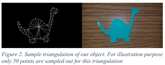
where N is the number of points on the contours. We also sample out 500 points for triangulation. |
|
Delaunay Triangulation:
|
|
|
Condition for Object detection:
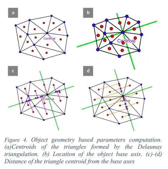
iv. This forms the base x axis and the axis perpendicular
to it forms the base y axis. This is shown in Fig. 4(b)
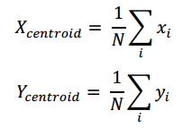
Once the base axis is set, the next step is to find the mean
normalised distance from the triangle centroid to the base axes.
|
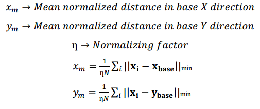
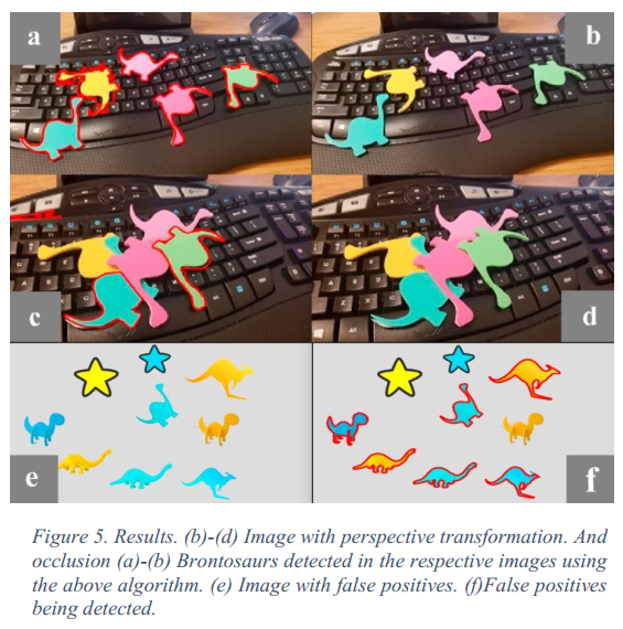
The above step is done for the model object and the range of the mean distances are set. The mean is divided by a normalizing factor in order to make it scale invariant. In our case we used the maximum distance from the centroid as the normalizing factor. This computed mean is used for comparison with the test image and the object detection is done. It was observed that the value of the mean normalized distance ranged from 0.4 to 0.8. It can be seen from the Fig. 5 that this method is robust to perspective transformation but not robust to occlusion. Higher the range of the mean normalized distance, higher is the is the probability of the object getting matched. However this increases the chance of false positives getting detected, as seen in the Fig. 5(e)(f) where a kangaroo with similar shape is being detected as the brontosaur |
|
|
[1] Pedro F. Felzenszwalb ‘Representation and Detection of Shapes in Images’, University of Chicago
|