This project aims at implementing EKF based online SLAM for mobile robots in indoor environment. We use data from 2D Lidar and wheel encoder to estimate the state of the robot and use EKF based filtering techniques to build a map. We would use ROS and Gazebo for simulation of our implementation.

The methodology followed is mentioned below:
• Give the input to the robot
• Collect the sensor data (LIDAR/odometry).
• Perform sensor fusion on the data
• Extract Features from the LIDAR Data
• Add new features into the database
• For existing features, send the position information to the kalman update step
• Calculate the kalman gain
• Calculate the new estimate based on previous estimate and measured value
• Update the map with the new information
• Do the above steps till the loop closure is attained
• Repeat the steps to improve the accuracy of the map

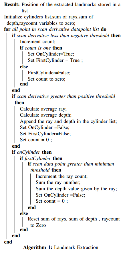
1. Landmark Extraction:
The simulator environment which we have created has cylindrical pillars as landmarks which should be extracted from the sensor data. Whenever there is a cylinder in the environment, the rays hitting the cylinder will have a range value different from the others. This changes can be found out by taking the derivatives of the sensor data and finding the spikes in the data.So,the derivatives of the sensor data are calculated at each instant and stored in a list. The start of the cylinder can be found by finding the negative spike whereas the end of the cylinder can be found out by positive spike. We should also consider the case of overlapping cylinders which might give multiple spikes. These edge cases also addressed in the algorithm given below. So, the Algorithm 1 explains the extraction of the landmark position by finding spikes in the environment

2. Extended Kalman Filter
The sensor data used for state estimation, being noisy, gives rise to accumulated errors. There are several techniques to reduce the error and one of the well established methods is to use recursive probabilistic filters. The Bayes filter is a recursive probabilistic filter which uses a prior belief and applies Bayes theorem to get a posterior estimate.

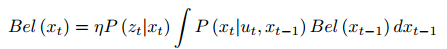
Kalman Filter is a variant of the Bayes filter where, the states are considered as a Gaussian distribution with a mean around the actual value and an uncertainty defined by the covariance. The problem with Kalman Filter is that it cannot be applied to non-linear systems. In order to use this methodology to non-linear systems, the system is linearized using Taylor’s expansion or Jacobian Linearization. This method is called Extended Kalman Filter.
The Extended Kalman Filter has two steps: (a) prediction step and (b) correction step. In the prediction step, the current state is predicted using the previous state and the current input. This gives us a belief of our current state with some uncertainty. This uncertainty is reduced after the correction step. In this step, sensor measurement data is used to correct our predicted belief. The prediction step is also called Motion Model and the correction step is also called Observation Model.